Inspecting the interior surface of a cylinder bore is one of the more geometrically constrained problems in machine vision. The camera has to see a curved surface through a circular aperture that's often smaller than the imaging distance you'd want. Lighting has to reach deep into the bore while producing enough contrast on the surface features you're trying to detect. Depth of field has to cover the bore depth, which is typically several times larger than the bore diameter. None of this is impossible, but each constraint interacts with the others in ways that take planning to handle.
This post works through the geometry and optics decisions for a cylinder bore inspection setup, using a representative engine component as the worked example. The target: a honed aluminum cylinder bore, 86mm bore diameter, 130mm depth, running on a transfer line at 45 parts per minute. Defects of interest include honing pattern irregularities, score marks from tooling, and bore roundness deviations visible as shadow patterns under axial illumination.
The fundamental constraint: working distance vs. field of view
The first question in any bore inspection setup is how much of the bore surface you need to see in a single frame. There are two basic optical strategies:
Axial view with a telecentric or long-working-distance lens: The camera looks down the bore axis. A single frame captures the bore entrance, and with careful focus stacking or a lens with sufficient depth of field, you can see the full cylindrical surface unwrapped into an annular image. The disadvantage is that axial lighting tends to pool at the bore centerline and leaves the sidewalls in shadow unless you use a ring light at steep enough angle to redirect light onto the bore wall.
Radial view with a fisheye or mirror-prism attachment: A borescope-style attachment bends the optical path 90 degrees so the camera looks radially at the bore wall. A single rotation or a fisheye optic captures the full circumference. The advantage is direct viewing of the bore wall surface with better spatial resolution. The disadvantage is that fisheye optics introduce significant radial distortion that must be corrected before the model sees the image.
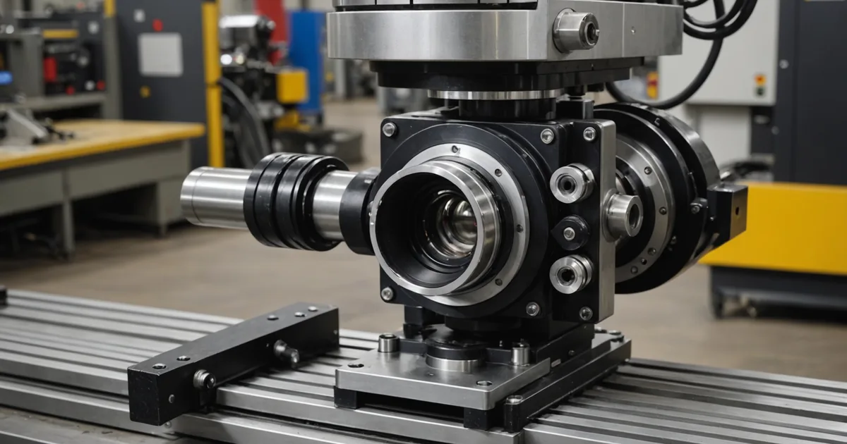
For the 86mm bore at 130mm depth, we used the axial approach with a coaxial illumination ring mounted at the bore entrance. The coaxial arrangement means light travels parallel to the optical axis into the bore and reflects off the bore wall back to the camera. Score marks and honing irregularities disrupt the expected reflection pattern and appear as dark or bright anomalies against the regular honing crosshatch background.
Depth of field calculation for the bore depth
Depth of field (DoF) is the range of distances from the lens that appear acceptably sharp in the image. For a bore 130mm deep with a camera positioned 200mm above the bore entrance, the focus target is the bore wall, which spans a depth range from roughly 0mm to 130mm from the bore entrance.
The thin lens formula relates object distance (u), focal length (f), and image distance (v): 1/f = 1/u + 1/v. For a GigE camera with a 1/2" sensor and a 25mm focal length lens focused at 250mm working distance, the depth of field at f/8 aperture is approximately 40mm. That's not enough to cover 130mm of bore depth in a single focus position.
There are three practical solutions:
- Focus bracketing: Take two or three frames at different focus positions and composite them, or run separate inference on each frame. This works but multiplies cycle time by the number of focus positions.
- Telephoto lens with smaller aperture: Longer focal length at higher f-stop (f/16 or f/22) increases DoF significantly, at the cost of requiring more illumination power to maintain exposure time. At f/16 with a 50mm lens at 350mm working distance on a 1/2" sensor, DoF increases to approximately 90-110mm — still short of 130mm but closer.
- Liquid lens or focal sweep: An electrically tunable liquid lens can sweep focus range in under 5ms, covering the full bore depth within a single part presentation window. This is the approach we use for deep bore applications — it adds hardware cost (~$180-$320 for the lens module) but eliminates the multi-frame complexity.
For the 45 ppm transfer line, cycle time per part is 1.33 seconds. With a liquid lens sweep taking 5ms per focus position and three positions covering the 130mm depth, total image acquisition time is under 20ms — well within the cycle time budget.
Illumination geometry for bore wall contrast
The surface feature that matters most on a honed bore is the honing crosshatch — the regular 45-degree scratch pattern left by the honing stones that creates the oil retention geometry. Defects present as disruptions to this pattern: missing crosshatch (indicates stones loaded or glazed), deep score marks crossing the pattern, and roundness deviation shadows where the bore wall has deviated from circular.
Coaxial illumination, where the light source is co-aligned with the optical axis via a beam splitter or ring, produces specular reflection from the bore wall. The honing crosshatch reflects diffusely in a different direction than the specular reflection, creating a characteristic bright-field image where the crosshatch appears darker than the surrounding bore wall. Score marks that cross the crosshatch at different angles appear as bright streaks against the darker crosshatch background.
Annular ring lights placed at the bore entrance at approximately 15 to 20 degrees from axial are an alternative to true coaxial illumination. They're simpler to mount and cheaper, but the illumination angle means the crosshatch contrast is less uniform across the bore depth — parts of the bore that are farther from the entrance receive light at steeper effective angles, which changes the apparent contrast of the same surface feature. This inconsistency increases the difficulty of the detection problem for the model and tends to produce more false positives at bore depths beyond 80mm.
We landed on a custom coaxial illumination module with a 72mm LED ring inside a telecentric shroud sized for the 86mm bore diameter. The shroud prevents ambient light from the transfer line from entering the optical path — bore inspection is particularly sensitive to ambient light variation because you're imaging a cavity that acts as a partial light trap.
Frame rate and part presentation window
At 45 ppm on a transfer line, parts are presented in fixed positions on a pallet — they stop, dwell for approximately 0.8 seconds at the inspection station, then advance. This is a significantly more tractable scenario than conveyor inspection, where the part is moving during image capture. The fixed dwell window means we can trigger image acquisition on the part-present signal from the PLC rather than using a motion-synchronized trigger.
With a 0.8-second dwell and three focus positions for full-depth coverage, we configure the system to capture images at focus positions 0ms, 12ms, and 24ms into the dwell period, leaving the remainder of the window for inference and PLC signal output. Inference on three frames in parallel takes approximately 18ms on the system's i7-12700 IPC. The reject signal is available well within the dwell window, giving the transfer line controller time to actuate the reject mechanism before part advance.
Model training considerations for bore images
Bore inspection images are unusual compared to flat-surface inspection: the input images have strong radial symmetry, a dark center region (the bore axis), and the defect region of interest is an annular band at a specific radius. Standard object detection models like the architecture Procunit uses will work on these images, but training data needs to capture the full range of bore depths and illumination conditions you'll encounter.
The most important training decision for bore inspection is whether to train on raw captured images or on images after a cylindrical unwrapping transform. Unwrapping converts the annular bore image into a rectangular strip representing the bore wall as if it had been cut and flattened. This makes the defect appearance more consistent across angular position and bore depth, which helps the model generalize. The tradeoff is that the unwrapping transform must be calibrated to the specific bore diameter and camera geometry — it's not a generic preprocessing step.
For the 86mm bore example, we used unwrapped images after calibration. The training set included 78 labeled defect examples (score marks, crosshatch anomalies, and two instances of bore roundness deviation visible as asymmetric shadow patterns) and 140 clean examples sampled across the full bore depth range. Training ran in approximately 4.5 hours overnight. The resulting model ran at under 8ms per frame on the deployed IPC.
Bore inspection is a harder setup problem than flat-surface inspection, but it's not a different category of problem. The same model architecture, the same training workflow, and the same PLC integration applies. The difference is that the optics and illumination require more careful upfront engineering, and the image preprocessing before the model sees the frame is more specific to the bore geometry. If you're working on a bore inspection application and want to talk through the geometry for your specific bore dimensions, reach out.